Transient Plotter...

 Astronomical transients have always been of special interest - the radio astronomy Vela pulsar observations searching for 'glitches' were motivated by this. Now activities have migrated over to optical astronomy and that interest in transients remain.

A subscription (free) to email alerts from the Transient Name Server (TNS) was made and alerts come in this format in an email...

The following new transient/s were reported on during the last day:

2024aazu RA=18:55:37.530, DEC=+01:30:48.46, Discovery date=2024-11-05 01:22:04.800, Discovery mag=14.42 ABMag, Filter: G - Gaia, Reporter: S.T. Hodgkin, E. Breedt, A. Delgado, D.L. Harrison, M. van Leeuwen, G. Rixon, T. Wevers, A. Yoldas ..., Reporting group: GaiaAlerts, Data source group: GaiaAlerts

2024aazw RA=20:15:22.890, DEC=+36:30:45.47, Discovery date=2024-11-04 09:51:50.400, Discovery mag=14.44 ABMag, Filter: G - Gaia, Reporter: S.T. Hodgkin, E. Breedt, A. Delgado, D.L. Harrison, M. van Leeuwen, G. Rixon, T. Wevers, A. Yoldas ..., Reporting group: GaiaAlerts, Data source group: GaiaAlerts

2024aazx RA=07:03:57.730, DEC=-02:12:37.22, Discovery date=2024-11-04 10:29:16.800, Discovery mag=13.3 ABMag, Filter: G - Gaia, Reporter: S.T. Hodgkin, E. Breedt, A. Delgado, D.L. Harrison, M. van Leeuwen, G. Rixon, T. Wevers, A. Yoldas ..., Reporting group: GaiaAlerts, Data source group: GaiaAlerts

The alert comes with the transient's ID, RA/DEC coordinates, discovery time, discovery magnitude, followed by other information.

Curiosity about the distribution of transients provided the motivation to code a rough plotting application (C# Windows GUI) which would accept a cut-and-paste of the transient/s information lines and parse them into names and RA/DEC coordinates.  The application then plots them on a RA/DEC graph which has a Hydrogen Line image as the background (which provides a guide to the position of the Milky Way).

As new transient alerts arrive they can be added to the list and the plot updated to show the new entries.

An example result is shown below...

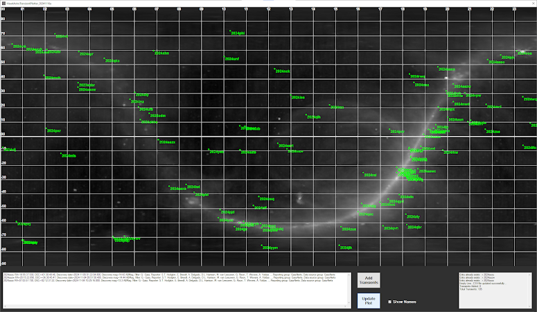
Typical Plot (~100 transients) with Names Shown

As can be seen as the number of transients increase there is confusion due to the names overlapping. An option to only plot the points is provided as shown below...

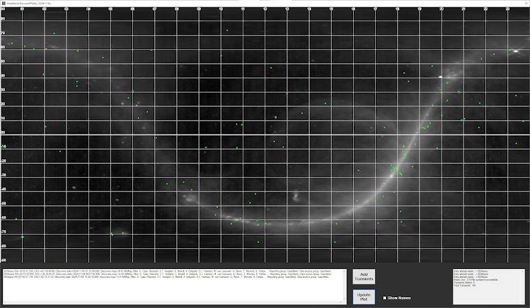
Typical Plot Without Names

As would be expected the highest density is near the Galactic Centre, but interestingly this density is - so far - not overwhelming higher than elsewhere.

It will be interesting to see how the plotting progresses over time as new transients are added.

Some extra functions may be added at a later date. For example - display only the newest object or objects for the purpose of seeing whether they can be seen in the Seestar S50.

NOTE: The TNS alerts come from telescopes which monitor a very large area of the sky. The likelihood of an amateur telescope with limited FOV discovering a transient are vanishingly small. Of course it is possible - but the likelihood of beating the professional observations is not great.

Observation Aid: SkyViewAltAz - Update #3

 When planning observation runs there is - unfortunately - a further factor that needs to be taken into account besides the visibility of targets through the various partial sky views available on the home block. That further factor is - of course - a clear sky.

While the application works well at its purpose of showing possible targets for the night, the presence of a clear sky was not included - which required looking up various websites.

The online website 'Clear Outside' provides a graphic which gives a forecast for the next couple of days in terms of skies suitable for observations. This graphic has been added to the 'SkyViewAltAz' application. Some re-arrangement of the GUI was also done to fit the graphic in.

Conveniently the 'Clear Outside' graphic is updated every hour and provides a prediction of cloud cover in general area of the home observatory.

Observation Aid: SkyViewAltAz - Update #2

Some added functionality and a bug fix. The added functionality extends the search function to actually select the object - if found - and display its data. Checkboxes are provided for a full data search (on by default) and also to 'lock' the found object - to allow changing the date and time without updating the drop-down object list. Some re-arranging and resizing of the search function text boxes has also been done.

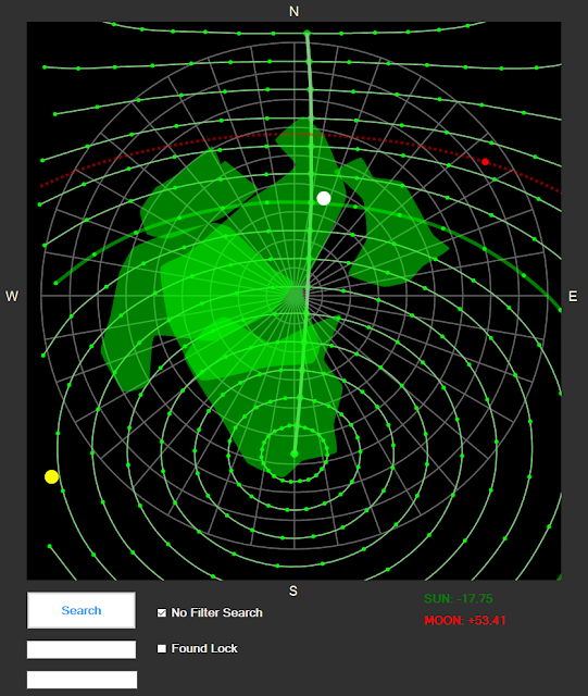
The position of the Sun and Moon are now calculated and representative filled circles (yellow for the Sun - white for the Moon) are plotted on the display. The current elevation of both of these objects is displayed (in green if below the horizon - red if above the horizon).

The bug fix prevents off-screen plotting (outside the PictureBox component) drawing spurious lines (see previous post image).  Instead of plotting the whole range at once, the plot points are tested to see if they are outside the PictureBox client rectangle and - if so - the segment up until that point is plotted.  Points are then continued to be scanned until a point is found inside the client rectangle and then the process repeats until all 'on-screen' points have been plotted. The granularity of the plotting points means that sometimes the plotted lines end before they have reached the edge of the PictureBox client rectangle - but this is considered the lesser of the two evils.

Another change is to the large image which is displayed on the right (nominally a screenshot from Stellarium) to indicate the size of the object w.r.t. the Seestar's FOV. As actual observations of an object are done, the object Stellarium screenshot will be replaced with an actual suitable Seestar observation image.

Apologies for the programming-oriented details. When the clouds stop coming over at night it will be back to pretty pictures...

Observation Aid: SkyViewAltAz - Update #1

 After evaluating the prototype version of SkyViewAltAz, a number of changes and additions were made. The intent is to provide a tool to assist in planning observation sessions - initially for use with the Seestar S50.

The current version provides time controls, selection of the various sky views from the home block (plotted on an Az/El grid), the path through the sky views for a selected object as well as various types of information (altitude/ azimuth, current field rotation, etc).

There are also filter options which limit which objects are populated in a drop down list, e.g., a range before and after LST, visibility in sky views - or visible from latitude 34 S (or no filters).

A thumbnail captured from the web (Wikipedia) is displayed to give an idea of the object itself - but of more use is a larger screenshot image (Stellarium) of the appearance of the object in the field of view (FOV) of the Seestar S50. This is very useful as images found on the web are the result from a wide variety of telescope FOVs - so, an object which looks like an interesting target judging from an image seen on the web might actually be from a large telescope with a very small FOV - but when viewed on a Seestar S50 may be just a dot in its much larger FOV.

SkyViewAzEl GUI (click on the image for a larger view)

All I need now is for the clouds to go away...

NOTE: the details provided here of SkyViewAzEl are informational only and primarily for my own documentation. Please don't ask for copies - I don't ever share my code as I have neither the time nor inclination to provide same - not to mention copyright issues (Wikipedia, Stellarium). To avoid being offended by a non-response - don't ask.

Observation Aid: SkyViewAltAz

As mentioned in a previous post - planning is fairly complex for observing on the home block. That post briefly described an application that was coded called "HawkAstroSkyView" - which mapped azimuth/altitude onto an RA/DEC grid. As explained, this greatly simplified planning - but provided a display dissimilar to the actual view when standing outside. To address this issue another application was coded called "SkyViewAltAz" where the altitude/azimuth sky 'patches' are mapped onto an alt/az 'dome'. The alt/az grid is overlayed with a RA/DEC grid. The alt/az grid 'dome' view more closely matches the view when standing outside - while the RA/DEC indicates the path through the sky view patches.  The RA/DEC is marked with dots spaced one hour apart. Note that all sky view patches are coloured green instead of individual colours and all can be viewed at one time (which allows determination whether the desired target object is visible in any sky view) - or individual views can be selected on their own to show detail of that particular sky view.

Buttons are provided to set date and time as for the previous application. This allows building observation plans for particular target objects by identifying the time of year where the object is visible overhead. For example - on this home block January-March is the best time of the year to start observing M42 around 8 pm in the evening. To observe now (end of September) the observation would need to start at around 2 am in the morning.

An enhancement which might be useful is to overlay a 'heatmap' of the degree of field rotation for the alt/az 'dome'. This may help identify pointings where the default exposure time can be increased from the nominal 10 seconds. That function may be added in the future.

Todmorden Pier - Variation...

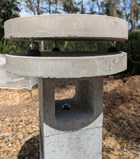
The semi-permanent pier design is based on the Todmorden Pier. It comprises an assembly of concrete pavers and 'Besser' concrete blocks with furniture level adjusters. Construction adhesive for concrete was used to glue various parts to one another.

From the bottom up the components are...

1. 600mm x 600mm x 25mm square concrete square.
2. 400mm x 50mm round concrete paver (under shimmed at 3 points with thin rubber washers to roughly correct for slope of the underlying square paver).
   Note that these first 2 pavers are not affixed to each other.
3. Two 'Besser' concrete blocks. The first block is glued to both the round paver below and the second block above it.
4. A third 'Besser' block bolted to the second block below it. It is bolted instead of glued to allow the pier to be broken down into sections for easier transport - if needed.
5. 400mm x 50mm round concrete paver. This round paver is glued to the third 'Besser' block below it.
6. A set of three 8mm diameter furniture levellers are fitted at 120 degrees intervals. Holes (10mm) were drilled in the top 400mm x 50mm round concrete paver to accommodate the threaded portions of the levellers. There was found to be too much slop and the next iteration will use 8mm holes worked to just allow fitment of the 8mm diameter leveller shanks.
7. Last 400mm x 50mm round concrete paver on top provides the mounting table for the smart telescopes (but also allows placement of the mount for a Celestron 4SE telescope).

Levelling of the top round paver is done by adjusting the top nut of each of the levellers whilst monitoring the level on the small smart telescope tripod. The levellers and top round paver are not glued and rely on gravity to keep them in place - the weight being sufficient for this. However, consideration will be given to whether to glue the bottom of the levellers to the underlying round paver. This would make assembling the top round paver simpler - but great care would needed to ensure proper alignment with the top round paver is achieved before the glue hardens.

This setup allows quick setting up of the smart telescopes and provides means to correct for any drift from the horizontal level due to ground movement.

After testing for a period of time, additional piers will be placed around strategic positions on the block. Each pier costs around $AUD 75.

The positions of those additional piers will be determined by mapping the sky view of candidate locations on the block in terms of points of azimuth and elevation. From those maps - with the help of custom coded applications - it can be determined whether a location warrants the construction of a pier of the design described above.

Observation Aid : HawkAstroSkyView

One of the disadvantages of our home block with regards to astrophotography is the tree coverage. There are just a handful of sites on the block which afford a clear sky view - and then only a small patch of the sky depending on the location. Trying to plan observing sessions is a hit-or-miss affair which involves wandering around trying to find a location where the target object is in view for the required time and duration of the observation.

To try and simplify this process an application was coded to plot an RA/DEC grid onto which is plotted objects - such as the Sun and Moon, the planets and a selection of deep sky objects (DSOs). Overlayed with that plot is colour-coded mapping of the azimuth/altitude views from a number of locations on the block.

Buttons are provided to adjust the date and time of the view and by adjusting these it's possible to plan when and where a target object may be observed. This simplified the planning process considerably !

The issue with this method of displaying the position of target objects is that the mapping of the azimuth/altitude windows on the sky produces a result which isn't easily visualised. The coloured areas so mapped don't agree with the actual view when standing outside and looking up.

Therefore - although this application greatly simplifies observation planning - it was decided to do the inverse where the parent grid is azimuth/altitude and an RA/DEC grid is mapped onto that. This produces a display more akin to the actual view as seen when standing outside. Should only take a week or two to code that.

Taking Stock...

It's been a while since posting - but as more experience and knowledge is gained with regards to astrophotography, the amount of information and options becomes overwhelming. What was needed was time to sort out just what are the activities that have the greatest interest to me and try and focus on them. Otherwise it becomes too confusing.

So - time was taken to take stock and try and lay out a broad scenario of activities for the foreseeable future.

Although efforts have been made to narrow-down activities, the wide range available only allows a general plan of attack. Activities - in the short term - will be guided by these broad factors.

• I have little interest in spending time and money to strive for the best possible result. Rather I want to use available time to learn about the night sky.
• I do not like many of the high-end post-processing results I've seen - especially using AI. I have seen results where the AI algorithm has decided that something should look a certain way and added features which are not real. The high-end post-processing looks too much like 'cosmetics' for my taste - indeed I've seen results which could be described as 'lipstick on a pig'.
• Apart from casual visual observing, I have no interest in assembling a very expensive astrophotography setup. I have found the use of my 'smart' telescopes (ZWO Seestar S50 and Dwarf II) entirely satisfactory for my level of activity. If I cannot set up in a few minutes and start observing I am not interested. Adding to the tedium of polar aligning a setup, the location here at home has restricted sky views due to trees. Consequently any form of permanent setup would need to be replicated in at least 5 or 6 places to provide access to a reasonable area of the sky. In addition the need to grab short periods of clear skies means the smart telescopes are much more suitable. I've seen claims by several individuals that they can setup and begin observing on their expensive assembled setup within 5 minutes - but no video proof is provided as far as I'm aware. I very much doubt anyone can carry out all the gear, assemble to a tripod, connect all the cables, polar align and begin observing in under 5 minutes.

I plan to take time to learn how to get the best out of the smart telescopes using minimal post-processing.

As a side interest I will switch my programming activities to various observation aids. The small patches of clear sky through the trees available on the home block makes planning complex. The process of determining which objects are visible from various locations is tedious and a time-waster. I'll code some applications which map the available sky areas and show the path of a given target object through those sky view windows.

To further reduce the setup time a variation of the 'Todmorden Pier' was prototyped. As the soil here is very reactive (moves due proximity to an escarpment and expands and contracts with moisture level) the digging of a deep hole for a concrete foundation was abandoned. Instead an assembly of concrete pavers and 'Besser' concrete blocks was built - to be described in the next post.

Matching the 'Look' Using CDFs and Final Tweaks...

 As an exercise I was interested to see how close an example Seestar S50 observation image could be processed to take on the 'look' of a target image.

As before a target image was loaded and a histogram applied to the Seestar S50 observation image data via a CDF (Cumulative Distribution Function) as shown below.

Histogram Matching Using CDFs

The target image 'look' is shown below in more detail...

Target Image for Matching to a 'Look'

It can be seen that the resulting matched image has the general look of the target image - but appears significantly de-saturated. To see if it is just a matter of de-saturation the resulting matched image was imported into GIMP and adjustments made to both saturation and colour temperature.

Before adjustment in GIMP...

Resulting Matched Image Before Adjustment in GIMP

... and after adjustment in GIMP...

Resulting Matched Image After adjustment in GIMP

Although the resulting matched observation image has a similar 'look' to the target image - it required manual adjustment (GIMP). Experiments will be done to determine whether examination of other statistics will allow automation of that adjustment.

Using CDFs to Histogram Match to an Existing 'Look'...

First Attempt

In the previous post which described automatically stretching via matching (using Cumulative Distribution Functions - CDFs) to mathematically generated red, green and blue channel histograms, mention was made of perhaps using existing good examples of the same object to provide a set of red, green and blue histograms.

I am interested how far the post-processing of Seestar S50 images can be automated. Accordingly, some code was written to implement the histogram matching function using good example images as shown below.

Histogram Matching to an Existing Good Example Image - Before Matching

PLEASE NOTE: the above application is just for experimental purposes and is not suitable for other use. Do not ask for a copy - unless you like being offended by a non-response :-)

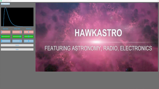
In this application the FITS observation file that is to be 'stretched' by histogram matching is loaded into the large image box. In the above picture the original linear image is shown. Then an example of an existing good stretched image of the same subject is loaded (the small image box top-left). Typically this might be images from the 'net from professional or amateur sources.

The application then calculates histograms of both the observation image file and the example stretched image file. After calculating CDFs from each histogram, the original linear image is re-mapped such that its histogram matches the good example image histogram.

The results of that process is shown below.

Histogram Matching to an Existing Good Example Image - After Matching

If we compare this result with the result from the previous post where the matching was done to a mathematically generated (via equations) as shown below (ignore the rotation), we can see that the above result has taken on the 'look' of the example image and is a better result as a consequence.

Comparison Result from Using a Mathematically Generated Histogram for Matching

If we choose a different example image which has a different 'look' and repeat the process we get the result as shown below.

Histogram Matching to a Different Existing Example Image (more blue)

Note the difference between the two example images in both cases (the small images top-left in the application). The second example has more of a blue-ish tinge than the first - so the result has the same elevated blue-ish tinge.

A further example uses an example image which has a completely different 'look'...

Histogram Matching to Radically Different 'Look' Example Image

In this example image there is more red and green and so the result of histogram matching takes on that 'look'. Other features to note is that for this M42 image, the detail around the trapezium in the result images matching the detail in the example images.  Where the trapezium detail is prominent in the example image, likewise it is prominent in the result. So - not only is the colouring of the example image adopted, but also the stretch curve shape.
I am pretty pleased with this result - which, once again, is better than I expected. Some notes...

• In the above results absolutely no manual tweaking is done. Just load in the observation file and the example image file and hit 'GO'. So - the above results - as far as processing is concerned - are obtained 100 % automatically.

• No spatial information is transferred from the example image (i.e., no matching of individual pixels is done). The spatial information is lost in the histogram calculation. It is simply the statistics (histogram and CDF) which are matched.

• The example images - used to match the observation image histogram to - are typically generated by a different camera (sensor), different post-processing applications, etc, and so the matching cannot be exact.

• Likewise - the exposure times for the example images is likely to be much longer (or the result of a larger aperture lens) and so the signal-to-noise ratios for the Seestar S50 images to be matched are likely to be much lower. Some compensation for this effect might be possible.

Further experimentation will be conducted to explore how far this technique can be extended.

Histogram Matching Using CDFs...

NOTE: the following histogram matching method is almost certainly not novel in the field of astrophotography post-processing given the amount of development effort put into processing applications. It is already used - for example, in medical imaging where images taken at different times and exposure conditions (leading to differences in contrast, brightness, etc) need to be compared to track changes.

It occurred to me (almost certainly not the first) that a similar histogram matching approach as used in medical imaging might be useful in order to circumvent the laborious manipulation normally associated with 'stretching' an astronomical image. Accordingly, I wrote some code to implement a histogram matching function.

Histogram Matching Application

PLEASE NOTE: the above application is just for experimental purposes and is not suitable for other use. Do not ask for a copy - unless you like being offended by a non-response :-)

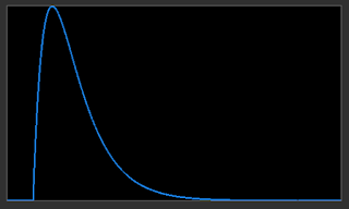
The application allowed the generation of a target histogram with various rise-times and delays in terms of their shapes. Two examples are given below...

Using Cumulative Distribution Functions to Match Histograms

The process is as follows...

1. Calculate histogram of original linear image. The data is processed in 16-bit unsigned values - so there are 65536 values in the histogram.
2. Calculate CDF of the linear histogram - also with 65536 values.
3. Calculate CDF of the generated target histogram (as displayed as examples above).
4. Create a re-mapping table by stepping through the linear image CDF values (for levels 0 - 65535) and reading out the CDF value. Then scan through the CDF of the generated target and find the nearest value to the linear CDF value. The index (0 - 65535) becomes the remapped value.
5. For every pixel in the linear image data, look up the entry in the re-mapping table which corresponds to its value and place in a matched image data set.
6. Display the matched image data.

No optimisation of speed nor determination of the most appropriate generated target histogram has been done. Just 'in principle' experiments.

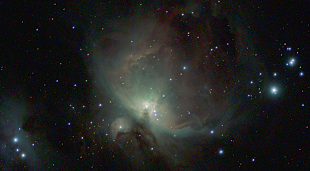
The result of matching the original linear image data (M42: 2.5 minutes integration Seestar S50) histogram to left-most example given above is shown below.

Result of Histogram Matching Using CDF of Generated Target Histogram

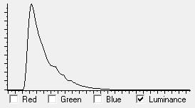
Comparing the generated target histogram against the histogram matched linear image shows a close match.

Target Histogram

Linear Data Histogram After Matching

Of note in the 'histogram matched' image is that the low-level nebulosity is visible at the same time as the high level detail (around the Trapezium) is preserved. This is a surprisingly good result. On the downside is the washed-out look in terms of colour. Just why is unknown at the time of writing.

Certainly this is a vast improvement over the previous first attempts at re-mapping using the CDF directly.

Some manipulation in GIMP results in the following image...

Result of Histogram Matched Image Processed by GIMP

I am pretty pleased with this result.

It may be possible to avoid trying to find the best generated target histogram by analysing good example images of targets and calculating the target histogram directly from those good example images. Perhaps a library of target histograms could be built making post-processing a simple exercise of auto stretching via CDFs with final tweaks in external programs such as GIMP as in the above example.

Interesting...

Histogram Matching...

As part of my experiments in astrophotography post-processing I noticed that - after applying a suitable non-linear stretch to the linear image data - the histograms of the stretched image had very similar shapes. As an example the histograms for an image of M42 are shown below.

M42 : Processed (Stretched) Image

The histograms for the luminance and the red, green and blue channels have been separately normalised to better show the similarity in shape. The relative amplitudes of the red, green and blue channels is shown below in the composite histogram plot.

Luminance	Red Channel
Green Channel	Blue Channel
Red, Green and Blue Channels Composite Plot

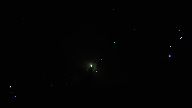
The original linear image as shown below where the pixel values are cramped down at the bottom end as shown in its luminance histogram.

M42: Original Unprocessed Linear Image

Original Linear Image Luminance Histogram

Implementing some way of modifying the data in the original linear image such that its histogram matches the shape and position of a stretched image histogram would be interesting. One way to do that is via "Histogram Matching" - the implementation of which will be described in the next post.

T Coronae Borealis - Recurrent Nova...

Took the opportunity of a clear sky to get a reference image of T Coronae Borealis using the Seestar S50 smart telescope. This is a recurrent nova with a burst period of about 80 years. There was a pre-cursor dimming last year leading to predictions it will go nova sometime this year (2024). Based on past observations it should brighten by a factor of about 1000.

If/when it goes bang I hope to get a comparison image.

Note (added 21 June 2024): I have noticed that in the above image there are 'phantom' stars at the 7 O'clock position next to the bright stars. This is - presumably - due to one or more misaligned sub-frames being added to the stacked image. At a later date a manual stacking process will be used to try and identify the misaligned sub-frames and remove them from the stack.

One-Shot-Colour (OSC) and Debayering...

The sensor in the Seestar S50 is a 'one-shot-colour' (OSC) sensor. Unlike a monochrome sensor - where each pixel in the sensor is a light bucket over a wide range of colours in the spectrum - the OSC sensor has colour filters (red, green and blue) placed over a group of 4 pixels in a 2x2 Bayer matrix. The pattern of filters can vary from sensor to sensor - but in the Seestar S50 the order is GRBG starting from the top-left pixel and moving right - then the second row left-most moving right.

Seestar S50 Bayer Matrix

Note that there are two green pixels in the group of four, with the remaining two red and blue. A number of characteristics arise from this.

• In an image of dimensions W x H, there are (W x H)/2 'green' pixels and (W x H)/4 'red' and 'blue' real physical pixels.
• With three colours in RGB colour space, this number needs to be 'rounded' up to 4 in order to form a symmetrical repeating pattern.
• Green is 'doubled-up' because of the history of OSC sensors is in normal photography and the eye is most sensitive to green.
• In order to provide a value of all three colours for every pixel, a de-bayering (de-mosaicing) algorithm is used. This is a process of generating values from adjacent pixels. There are different de-bayering algorithms and different Bayer matrix ordering. Therefore - when exporting non-debayered image data the Bayer matrix pattern must accompany the data.

In summary - for every 'real' red or 'blue' pixel there are two 'green' pixels. That is, the 'real' resolution for green is twice that of red or blue. This can be seen in the image data.

To illustrate that I've taken a small tile of an image (outlined in red) from the Seestar S50 and examined it in detail. The data is from an image which has been 'stretched' using a CDF (cumulative density function) as described here.

The tile shown below is 25 x 25 pixels and is taken from an area of noisy data. The image data is displayed starting with the RGB composite, then the red, green and blue component magnitudes in row/column order.

What is immediately obvious is that the spatial resolution is much better in the Green channel. The Red and Blue channels are more 'blobby'. In other words - there is more high frequency data (detail) in the Green channel versus the Red and Blue channels.

It can be seen that there are areas in the red and blue data where the level is 'black'. In the corresponding areas in the green data there is fine features. When combined into the RGB composite this is the source of the 'green noise'.

It is interesting to see the effects of 'modulating' the red and blue data with the higher resolution green data. The results are shown below.

Here more detail has been added to the red and blue channels by multiplying their original values by the green channel data. The effect on the original image is shown below.

There is significantly more 'sharpness' in the detail - albeit with corruption of the colour balance. Nonetheless I find this an intriguing result.

Unknown...

After taking a short exposure of NGC 3532 (Caldwell 91) I picked an area of nebulosity nearby via the inbuilt Seestar S50 'SkyAtlas'. It came up with 'Unknown' as there is no designated SkyAtlas object in that area. I found this fascinating where you can move around the sky in 'SkyAtlas' - pick something interesting and then tell the Seestar S50 to take an observation. If the Seestar S50 is a 'toy', give me more 'toys' like this...

Unknown :  11^h 13^m 58^s, −61° 20′ 40″

Billions and Billions of Stars...

As it was a rare clear night, after taking a long exposure of the Supernova in NGC 4216, I picked a target more southerly - an open star cluster called NGC 3532 (Caldwell 91). Despite only taking a 5 minute observation the number of stars seen is amazing ! I can hear Carl Sagan's voice - "billions and billions of stars..." The area of sky in the image has an angular width about the same as holding a pencil at arm's length.

NGC 3532 (Caldwell 91) : 11^h 05^m 12^s, −58° 44′ 1″

Minimalist Post-Processing...

Background

Having started learning about astrophotography at the beginning of 2024, it's been a bit of a wander through the various astrophotography 'rooms' trying different things. Each 'room' had its own attractions - but there are a great number of rooms.  There is also a lot of 'advice' as to how, what and where astrophotography should be done. It is easy to be restrained from picking your own 'niche'.

A comment often heard from some quarters is 'why do astrophotography ?' After all, much better images could be downloaded from the 'net captured by professional telescopes. That's true - but that is missing the most important point (at least for me) - which is - those images are not my images. The wonderment that the photons from some object millions of light-years away have been captured in my backyard telescope and converted to pixels in my image is missing from a downloaded image.

I'm gradually finding my own 'niche' guided by some parameters...

• I know next to nothing about the night sky.
• Viewing through an eyepiece is not an option due to eyesight and posture issues.
• Polar aligning an equatorial mount is not an option due to eyesight, posture and light pollution (SCP doesn't have a Polaris). I tried and could never do it.
• Spending hours on post-processing with clever - but complicated - post-processing applications is not my idea of fun.
• My sky view is limited to the home block being almost covered by tall eucalypts and so about a 1/2 dozen different sites on the block are needed to get some coverage. Therefore, a permanent installation is not practicable.

So - for my situation the Seestar S50 is the best telescope option. It makes the time taken to find and observe targets amazingly short. In fact, within 5 minutes from walking out the door with Seestar S50 you can be acquiring data.

Post-Processing Pain

Spending hours post-processing the data to get the 'best' picture (the definition of which is not agreed upon anyway) - for me - slowly drains the wonderment and fun out of the exercise.

To this end I have spent a lot of time writing code to analyse the FITS format files output from the Seestar S50 for the purpose of perhaps coming up with a way to automatically post-process the data into an acceptable image. This exercise was largely successful - but still requires too much manual intervention.

Seestar S50 to the Rescue

One of the fantastic aspects of the Seestar S50 is the regular updates to the phone application and onboard Seestar S50 firmware. There are so many enhancements that cool new features/functions are easily overlooked. One of the cool new functions I overlooked is called 'Deep Sky Stacker'. Previously the exposures were stacked on the fly while the observation is in progress producing a single stacked FITS and a 'thin' JPG (really just a thumbnail). The functionality has now been extended such that - if the option is checked in 'Advanced Feature' - all the single RAW FITS exposure files are saved also. In Deep Sky Stacker all - or a subset - of those exposure files can be selected and stacked. Maybe there are some satellite trails on some of them - so these exposures can be excluded from the stack. You can even stack images taken of the same object taken on different nights - provided the hour angles are roughly the same.

In addition, the stacked image can be edited in-situ, with controls for denoising, brightness, contrast and saturation. The images can be 'downloaded' immediately to the phone - or exporting to Google Drive or Dropbox (but exporting is delayed until the phone is disconnected from the Seestar S50 and normal WiFi access is restored).

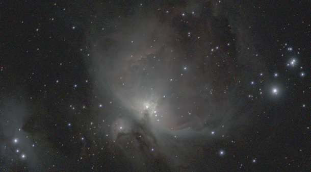
Below is an image of the Orion Nebula which has been processed entirely with the Seestar S50 phone app and the Seestar S50 firmware. I'm pretty happy with the result.

Orion Nebula (M42) Processed Entirely with the Seestar S50 Phone App and Onboard Firmware

I will explore this functionality further.

Supernova SN2024gy in NGC 4216 Fading...

 Took advantage of a - mostly - clear sky last night to re-observe NGC 4216 using the Seestar S50 smart telescope to see how much the supernova (SN2024gy) had faded. The comparison below shows the difference between its brightness some 2 and a bit months ago at 11th March 2024 compared to last night at 28th May 2024.

Supernova SN2024gy in NGC 4216 - Left 11 March 2024: Right 28 May 2024

It can be seen that the supernova (near the top of the upper 'wing') has faded significantly - but is still faintly visible.

Fascinating !

Using the CDF in RGB Colour Space...

Examination of the CDF in the graph below of a simulated astronomical image reveals that the shape of the CDF closely resembles the shape of typical non-linear 'stretch' curves used in astronomical image processing applications. It's an interesting exercise to use the CDF to remap the magnitude values according to the CDF.

In this example the magnitude values range from 0 - 100 (X-axis). Taking a magnitude value of 10 on the X-axis (10 % of full magnitude) and travelling up from 0 on the Y-axis - we cross the CDF at a PDF value of about 0.6 (right Y-axis).  Scaling this PDF w.r.t. to the full magnitude of 100 gives a value of 60. So - using the CDF we have remapped a magnitude value of 10 to a value of 60. This has the effect of spreading the low level detail further up the magnitude scale lifting it up out of the dark. Of course, this is a crude example - but nonetheless illustrates the principle.

PDF and CDF of a Simulated Astronomical Image

The effects of using this simple 'stretch' algorithm on three astronomical  image types is shown below - where individual CDFs are generated for each of the three RGB channels. The underlying data hidden in the linear view are revealed. The flaws in this simple stretch method are discussed.

First, the Horsehead Nebula (IC 434) - a somewhat faint nebula near a very bright star...

IC434 (Horsehead Nebula) with Simple CDF Stretch

The observation time was a short 12 minutes and so the nebula is faint and close to the noise floor. The faint details are brought up out of darkness - but at the expense of the bright parts - which are 'flattened' and devoid of detail. The stars appear bloated. The image also appears to be de-saturated in the bright parts.

The luminance histogram after this stretch indicates that using the CDF is a form of histogram equalisation - where values clustered down at the bottom of the magnitude scale are promoted up the scale. This is generally what is needed - but it is obvious that this simple method is not even close to ideal.

Second, NGC 4216 - a galaxy (with supernova) in a sparse star field with low nebulosity...

NGC 4216 with Simple CDF Stretch

Once again the bright parts are 'flattened' and devoid of detail. The stars again appear bloated. The image also again appears to be de-saturated in the bright parts.

The luminance histogram after this stretch indicates a form of histogram equalisation - where values clustered down at the bottom of the magnitude scale are promoted up the scale.

Third, the Orion nebula (M42) - a bright nebula with faint details covering a wide dynamic range...

Orion Nebula (M42) with Simple CDF Stretch

Once again the bright parts are 'flattened' and devoid of detail. The stars again appear bloated. The image also again appears to be de-saturated in the bright parts. The bright parts of the nebula cover a significant portion of the image.

Due to the predominance of bright nebulosity in this data, the histogram is closer to what is required. However, the bright parts still have little detail and are desaturated.

Another issue with this simple method is the that quantisation of the data is emphasised as shown in the histogram for just one colour - red.

The deviation from a more continuous curve is because when the re-mapping of values is done using the CDF, an increment of 1 in the input range resolves to many steps in the output range.  For example, using the CDF of the M42 image results in an input value of 600 to be re-mapped to 4837, while an increment of 1 in the input value to 601 is re-mapped to 5648. That means output values in the range 4838 to 5647 are not possible. This is not good as effectively many bits of amplitude resolution have been lost in the majority of the amplitude range - losing subtle detail.

Ways of reducing these flaws need to be found - if possible...