Matching the 'Look' Using CDFs and Final Tweaks...

 As an exercise I was interested to see how close an example Seestar S50 observation image could be processed to take on the 'look' of a target image.

As before a target image was loaded and a histogram applied to the Seestar S50 observation image data via a CDF (Cumulative Distribution Function) as shown below.

Histogram Matching Using CDFs

The target image 'look' is shown below in more detail...

Target Image for Matching to a 'Look'

It can be seen that the resulting matched image has the general look of the target image - but appears significantly de-saturated. To see if it is just a matter of de-saturation the resulting matched image was imported into GIMP and adjustments made to both saturation and colour temperature.

Before adjustment in GIMP...

Resulting Matched Image Before Adjustment in GIMP

... and after adjustment in GIMP...

Resulting Matched Image After adjustment in GIMP

Although the resulting matched observation image has a similar 'look' to the target image - it required manual adjustment (GIMP). Experiments will be done to determine whether examination of other statistics will allow automation of that adjustment.

Using CDFs to Histogram Match to an Existing 'Look'...

First Attempt

In the previous post which described automatically stretching via matching (using Cumulative Distribution Functions - CDFs) to mathematically generated red, green and blue channel histograms, mention was made of perhaps using existing good examples of the same object to provide a set of red, green and blue histograms.

I am interested how far the post-processing of Seestar S50 images can be automated. Accordingly, some code was written to implement the histogram matching function using good example images as shown below.

Histogram Matching to an Existing Good Example Image - Before Matching

PLEASE NOTE: the above application is just for experimental purposes and is not suitable for other use. Do not ask for a copy - unless you like being offended by a non-response :-)

In this application the FITS observation file that is to be 'stretched' by histogram matching is loaded into the large image box. In the above picture the original linear image is shown. Then an example of an existing good stretched image of the same subject is loaded (the small image box top-left). Typically this might be images from the 'net from professional or amateur sources.

The application then calculates histograms of both the observation image file and the example stretched image file. After calculating CDFs from each histogram, the original linear image is re-mapped such that its histogram matches the good example image histogram.

The results of that process is shown below.

Histogram Matching to an Existing Good Example Image - After Matching

If we compare this result with the result from the previous post where the matching was done to a mathematically generated (via equations) as shown below (ignore the rotation), we can see that the above result has taken on the 'look' of the example image and is a better result as a consequence.

Comparison Result from Using a Mathematically Generated Histogram for Matching

If we choose a different example image which has a different 'look' and repeat the process we get the result as shown below.

Histogram Matching to a Different Existing Example Image (more blue)

Note the difference between the two example images in both cases (the small images top-left in the application). The second example has more of a blue-ish tinge than the first - so the result has the same elevated blue-ish tinge.

A further example uses an example image which has a completely different 'look'...

Histogram Matching to Radically Different 'Look' Example Image

In this example image there is more red and green and so the result of histogram matching takes on that 'look'. Other features to note is that for this M42 image, the detail around the trapezium in the result images matching the detail in the example images.  Where the trapezium detail is prominent in the example image, likewise it is prominent in the result. So - not only is the colouring of the example image adopted, but also the stretch curve shape.
I am pretty pleased with this result - which, once again, is better than I expected. Some notes...

• In the above results absolutely no manual tweaking is done. Just load in the observation file and the example image file and hit 'GO'. So - the above results - as far as processing is concerned - are obtained 100 % automatically.

• No spatial information is transferred from the example image (i.e., no matching of individual pixels is done). The spatial information is lost in the histogram calculation. It is simply the statistics (histogram and CDF) which are matched.

• The example images - used to match the observation image histogram to - are typically generated by a different camera (sensor), different post-processing applications, etc, and so the matching cannot be exact.

• Likewise - the exposure times for the example images is likely to be much longer (or the result of a larger aperture lens) and so the signal-to-noise ratios for the Seestar S50 images to be matched are likely to be much lower. Some compensation for this effect might be possible.

Further experimentation will be conducted to explore how far this technique can be extended.

Histogram Matching Using CDFs...

NOTE: the following histogram matching method is almost certainly not novel in the field of astrophotography post-processing given the amount of development effort put into processing applications. It is already used - for example, in medical imaging where images taken at different times and exposure conditions (leading to differences in contrast, brightness, etc) need to be compared to track changes.

It occurred to me (almost certainly not the first) that a similar histogram matching approach as used in medical imaging might be useful in order to circumvent the laborious manipulation normally associated with 'stretching' an astronomical image. Accordingly, I wrote some code to implement a histogram matching function.

Histogram Matching Application

PLEASE NOTE: the above application is just for experimental purposes and is not suitable for other use. Do not ask for a copy - unless you like being offended by a non-response :-)

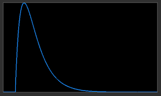
The application allowed the generation of a target histogram with various rise-times and delays in terms of their shapes. Two examples are given below...

Using Cumulative Distribution Functions to Match Histograms

The process is as follows...

1. Calculate histogram of original linear image. The data is processed in 16-bit unsigned values - so there are 65536 values in the histogram.
2. Calculate CDF of the linear histogram - also with 65536 values.
3. Calculate CDF of the generated target histogram (as displayed as examples above).
4. Create a re-mapping table by stepping through the linear image CDF values (for levels 0 - 65535) and reading out the CDF value. Then scan through the CDF of the generated target and find the nearest value to the linear CDF value. The index (0 - 65535) becomes the remapped value.
5. For every pixel in the linear image data, look up the entry in the re-mapping table which corresponds to its value and place in a matched image data set.
6. Display the matched image data.

No optimisation of speed nor determination of the most appropriate generated target histogram has been done. Just 'in principle' experiments.

The result of matching the original linear image data (M42: 2.5 minutes integration Seestar S50) histogram to left-most example given above is shown below.

Result of Histogram Matching Using CDF of Generated Target Histogram

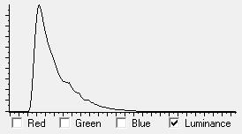
Comparing the generated target histogram against the histogram matched linear image shows a close match.

Target Histogram

Linear Data Histogram After Matching

Of note in the 'histogram matched' image is that the low-level nebulosity is visible at the same time as the high level detail (around the Trapezium) is preserved. This is a surprisingly good result. On the downside is the washed-out look in terms of colour. Just why is unknown at the time of writing.

Certainly this is a vast improvement over the previous first attempts at re-mapping using the CDF directly.

Some manipulation in GIMP results in the following image...

Result of Histogram Matched Image Processed by GIMP

I am pretty pleased with this result.

It may be possible to avoid trying to find the best generated target histogram by analysing good example images of targets and calculating the target histogram directly from those good example images. Perhaps a library of target histograms could be built making post-processing a simple exercise of auto stretching via CDFs with final tweaks in external programs such as GIMP as in the above example.

Interesting...

Minimalist Post-Processing...

Background

Having started learning about astrophotography at the beginning of 2024, it's been a bit of a wander through the various astrophotography 'rooms' trying different things. Each 'room' had its own attractions - but there are a great number of rooms.  There is also a lot of 'advice' as to how, what and where astrophotography should be done. It is easy to be restrained from picking your own 'niche'.

A comment often heard from some quarters is 'why do astrophotography ?' After all, much better images could be downloaded from the 'net captured by professional telescopes. That's true - but that is missing the most important point (at least for me) - which is - those images are not my images. The wonderment that the photons from some object millions of light-years away have been captured in my backyard telescope and converted to pixels in my image is missing from a downloaded image.

I'm gradually finding my own 'niche' guided by some parameters...

• I know next to nothing about the night sky.
• Viewing through an eyepiece is not an option due to eyesight and posture issues.
• Polar aligning an equatorial mount is not an option due to eyesight, posture and light pollution (SCP doesn't have a Polaris). I tried and could never do it.
• Spending hours on post-processing with clever - but complicated - post-processing applications is not my idea of fun.
• My sky view is limited to the home block being almost covered by tall eucalypts and so about a 1/2 dozen different sites on the block are needed to get some coverage. Therefore, a permanent installation is not practicable.

So - for my situation the Seestar S50 is the best telescope option. It makes the time taken to find and observe targets amazingly short. In fact, within 5 minutes from walking out the door with Seestar S50 you can be acquiring data.

Post-Processing Pain

Spending hours post-processing the data to get the 'best' picture (the definition of which is not agreed upon anyway) - for me - slowly drains the wonderment and fun out of the exercise.

To this end I have spent a lot of time writing code to analyse the FITS format files output from the Seestar S50 for the purpose of perhaps coming up with a way to automatically post-process the data into an acceptable image. This exercise was largely successful - but still requires too much manual intervention.

Seestar S50 to the Rescue

One of the fantastic aspects of the Seestar S50 is the regular updates to the phone application and onboard Seestar S50 firmware. There are so many enhancements that cool new features/functions are easily overlooked. One of the cool new functions I overlooked is called 'Deep Sky Stacker'. Previously the exposures were stacked on the fly while the observation is in progress producing a single stacked FITS and a 'thin' JPG (really just a thumbnail). The functionality has now been extended such that - if the option is checked in 'Advanced Feature' - all the single RAW FITS exposure files are saved also. In Deep Sky Stacker all - or a subset - of those exposure files can be selected and stacked. Maybe there are some satellite trails on some of them - so these exposures can be excluded from the stack. You can even stack images taken of the same object taken on different nights - provided the hour angles are roughly the same.

In addition, the stacked image can be edited in-situ, with controls for denoising, brightness, contrast and saturation. The images can be 'downloaded' immediately to the phone - or exporting to Google Drive or Dropbox (but exporting is delayed until the phone is disconnected from the Seestar S50 and normal WiFi access is restored).

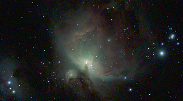
Below is an image of the Orion Nebula which has been processed entirely with the Seestar S50 phone app and the Seestar S50 firmware. I'm pretty happy with the result.

Orion Nebula (M42) Processed Entirely with the Seestar S50 Phone App and Onboard Firmware

I will explore this functionality further.