Unknown...

After taking a short exposure of NGC 3532 (Caldwell 91) I picked an area of nebulosity nearby via the inbuilt Seestar S50 'SkyAtlas'. It came up with 'Unknown' as there is no designated SkyAtlas object in that area. I found this fascinating where you can move around the sky in 'SkyAtlas' - pick something interesting and then tell the Seestar S50 to take an observation. If the Seestar S50 is a 'toy', give me more 'toys' like this...

Unknown :  11^h 13^m 58^s, −61° 20′ 40″

Billions and Billions of Stars...

As it was a rare clear night, after taking a long exposure of the Supernova in NGC 4216, I picked a target more southerly - an open star cluster called NGC 3532 (Caldwell 91). Despite only taking a 5 minute observation the number of stars seen is amazing ! I can hear Carl Sagan's voice - "billions and billions of stars..." The area of sky in the image has an angular width about the same as holding a pencil at arm's length.

NGC 3532 (Caldwell 91) : 11^h 05^m 12^s, −58° 44′ 1″

Minimalist Post-Processing...

Background

Having started learning about astrophotography at the beginning of 2024, it's been a bit of a wander through the various astrophotography 'rooms' trying different things. Each 'room' had its own attractions - but there are a great number of rooms.  There is also a lot of 'advice' as to how, what and where astrophotography should be done. It is easy to be restrained from picking your own 'niche'.

A comment often heard from some quarters is 'why do astrophotography ?' After all, much better images could be downloaded from the 'net captured by professional telescopes. That's true - but that is missing the most important point (at least for me) - which is - those images are not my images. The wonderment that the photons from some object millions of light-years away have been captured in my backyard telescope and converted to pixels in my image is missing from a downloaded image.

I'm gradually finding my own 'niche' guided by some parameters...

• I know next to nothing about the night sky.
• Viewing through an eyepiece is not an option due to eyesight and posture issues.
• Polar aligning an equatorial mount is not an option due to eyesight, posture and light pollution (SCP doesn't have a Polaris). I tried and could never do it.
• Spending hours on post-processing with clever - but complicated - post-processing applications is not my idea of fun.
• My sky view is limited to the home block being almost covered by tall eucalypts and so about a 1/2 dozen different sites on the block are needed to get some coverage. Therefore, a permanent installation is not practicable.

So - for my situation the Seestar S50 is the best telescope option. It makes the time taken to find and observe targets amazingly short. In fact, within 5 minutes from walking out the door with Seestar S50 you can be acquiring data.

Post-Processing Pain

Spending hours post-processing the data to get the 'best' picture (the definition of which is not agreed upon anyway) - for me - slowly drains the wonderment and fun out of the exercise.

To this end I have spent a lot of time writing code to analyse the FITS format files output from the Seestar S50 for the purpose of perhaps coming up with a way to automatically post-process the data into an acceptable image. This exercise was largely successful - but still requires too much manual intervention.

Seestar S50 to the Rescue

One of the fantastic aspects of the Seestar S50 is the regular updates to the phone application and onboard Seestar S50 firmware. There are so many enhancements that cool new features/functions are easily overlooked. One of the cool new functions I overlooked is called 'Deep Sky Stacker'. Previously the exposures were stacked on the fly while the observation is in progress producing a single stacked FITS and a 'thin' JPG (really just a thumbnail). The functionality has now been extended such that - if the option is checked in 'Advanced Feature' - all the single RAW FITS exposure files are saved also. In Deep Sky Stacker all - or a subset - of those exposure files can be selected and stacked. Maybe there are some satellite trails on some of them - so these exposures can be excluded from the stack. You can even stack images taken of the same object taken on different nights - provided the hour angles are roughly the same.

In addition, the stacked image can be edited in-situ, with controls for denoising, brightness, contrast and saturation. The images can be 'downloaded' immediately to the phone - or exporting to Google Drive or Dropbox (but exporting is delayed until the phone is disconnected from the Seestar S50 and normal WiFi access is restored).

Below is an image of the Orion Nebula which has been processed entirely with the Seestar S50 phone app and the Seestar S50 firmware. I'm pretty happy with the result.

Orion Nebula (M42) Processed Entirely with the Seestar S50 Phone App and Onboard Firmware

I will explore this functionality further.

Supernova SN2024gy in NGC 4216 Fading...

 Took advantage of a - mostly - clear sky last night to re-observe NGC 4216 using the Seestar S50 smart telescope to see how much the supernova (SN2024gy) had faded. The comparison below shows the difference between its brightness some 2 and a bit months ago at 11th March 2024 compared to last night at 28th May 2024.

Supernova SN2024gy in NGC 4216 - Left 11 March 2024: Right 28 May 2024

It can be seen that the supernova (near the top of the upper 'wing') has faded significantly - but is still faintly visible.

Fascinating !

Using the CDF in RGB Colour Space...

Examination of the CDF in the graph below of a simulated astronomical image reveals that the shape of the CDF closely resembles the shape of typical non-linear 'stretch' curves used in astronomical image processing applications. It's an interesting exercise to use the CDF to remap the magnitude values according to the CDF.

In this example the magnitude values range from 0 - 100 (X-axis). Taking a magnitude value of 10 on the X-axis (10 % of full magnitude) and travelling up from 0 on the Y-axis - we cross the CDF at a PDF value of about 0.6 (right Y-axis).  Scaling this PDF w.r.t. to the full magnitude of 100 gives a value of 60. So - using the CDF we have remapped a magnitude value of 10 to a value of 60. This has the effect of spreading the low level detail further up the magnitude scale lifting it up out of the dark. Of course, this is a crude example - but nonetheless illustrates the principle.

PDF and CDF of a Simulated Astronomical Image

The effects of using this simple 'stretch' algorithm on three astronomical  image types is shown below - where individual CDFs are generated for each of the three RGB channels. The underlying data hidden in the linear view are revealed. The flaws in this simple stretch method are discussed.

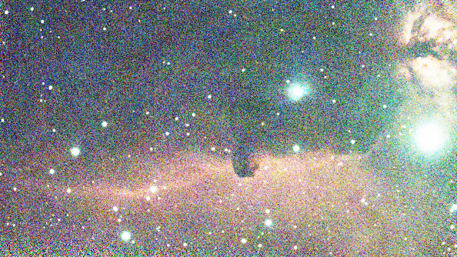
First, the Horsehead Nebula (IC 434) - a somewhat faint nebula near a very bright star...

IC434 (Horsehead Nebula) with Simple CDF Stretch

The observation time was a short 12 minutes and so the nebula is faint and close to the noise floor. The faint details are brought up out of darkness - but at the expense of the bright parts - which are 'flattened' and devoid of detail. The stars appear bloated. The image also appears to be de-saturated in the bright parts.

The luminance histogram after this stretch indicates that using the CDF is a form of histogram equalisation - where values clustered down at the bottom of the magnitude scale are promoted up the scale. This is generally what is needed - but it is obvious that this simple method is not even close to ideal.

Second, NGC 4216 - a galaxy (with supernova) in a sparse star field with low nebulosity...

NGC 4216 with Simple CDF Stretch

Once again the bright parts are 'flattened' and devoid of detail. The stars again appear bloated. The image also again appears to be de-saturated in the bright parts.

The luminance histogram after this stretch indicates a form of histogram equalisation - where values clustered down at the bottom of the magnitude scale are promoted up the scale.

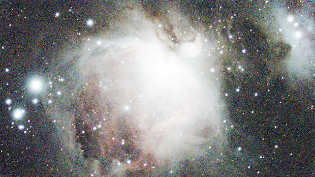
Third, the Orion nebula (M42) - a bright nebula with faint details covering a wide dynamic range...

Orion Nebula (M42) with Simple CDF Stretch

Once again the bright parts are 'flattened' and devoid of detail. The stars again appear bloated. The image also again appears to be de-saturated in the bright parts. The bright parts of the nebula cover a significant portion of the image.

Due to the predominance of bright nebulosity in this data, the histogram is closer to what is required. However, the bright parts still have little detail and are desaturated.

Another issue with this simple method is the that quantisation of the data is emphasised as shown in the histogram for just one colour - red.

The deviation from a more continuous curve is because when the re-mapping of values is done using the CDF, an increment of 1 in the input range resolves to many steps in the output range.  For example, using the CDF of the M42 image results in an input value of 600 to be re-mapped to 4837, while an increment of 1 in the input value to 601 is re-mapped to 5648. That means output values in the range 4838 to 5647 are not possible. This is not good as effectively many bits of amplitude resolution have been lost in the majority of the amplitude range - losing subtle detail.

Ways of reducing these flaws need to be found - if possible...

Histograms, PDFs, CDFs...

Histograms 

One of the most important tools for analysing astronomical images is the histogram. The histogram of the unprocessed astronomical linear image data shows clearly that the bulk of the pixels are cramped down at the bottom end of the magnitude scale as shown previously.

Example Astronomical Image Luminance Histogram

Also it was shown that the target for processing the image should spread the data values such that the bulk of the values lies around the 20 % - 25 % of the scale as shown below in the histogram of the 'everyday' image.

Everyday Image Luminance Histogram

This is done by 'stretching' the data, where the data values down near the bottom are increased, while at the same time the bright values near the top are left as they are. The stretching is done by some chosen non-linear function - but what and how ?

Recapping on the previous post concerning the form of the image data contained in stacked FITS files from the Seestar S50 - the data covers a range of an unsigned short integer (16-bits), that is, 0 - 65535. The histogram could have a bin size of  256 (as the histograms above have) - giving 256 separate bins. However, as the original linear data has been shown to be cramped down to the bottom few % of the magnitude, it is better to have a bin size of the value resolution, i.e., 1.  Therefore, there are 65536 bins.

To create the histogram then entails creating an array of 65536 elements each holding an integer count. The array type needs to be an unsigned 32-bit integer (range 0 - 4,294,967,296) to ensure there is enough range for counts in an image of 1080 x 1920 pixels (if all the pixels were full white, then the count in one bin would be 1080 x 1920 = 2,073,600).

For a Seestar S50 stacked FITS file, therefore, you would only need 21 bits unsigned (or 22 bits signed). However, the next step up after 16-bits is 32-bits. Of course, 32-bit signed integers could be used as halving the positive range down to 2,147,483,648 provides ample headroom - but personally (as all values will be positive) I prefer to use unsigned integers as that gives a clue in the code of the nature (i.e., all positive) of the data contained therein.

Building the histogram is simply a matter of reading each pixel in the image (three passes as there are three colours) and incrementing the value in the array element indexed by the value as read.

PDF - (Probability Density Function)

Not to be confused with the PDF document format, the Probability Density Function is a way of normalising the information contained in the image histogram. In the histogram, the Y-axis is the count of the number of pixels which have the value of the bin index. The scale of that count depends on the size of the image - a larger image will tend to have a higher count in each of the bins compared to a smaller image. By dividing the count in each bin by the total number of pixels in the image we get a normalised PDF with a Y-axis range of 0.0 to 1.0. Now for each magnitude value (X-axis) we get a probability of that value occurring in the image.

The use of the term 'probability' might seem a bit pretentious given the PDF just described is just a normalised count - probability is usually reserved for some random value. However, the term is justified. Imagine standing on a pixel somewhere in the image. The PDF gives the probability that any random pixel any distance away will be a certain value. As any random pixel must have a value in the magnitude range, the total of the individual probabilities for all magnitude values must equal 1.0.

Note that the shape of the PDF is the same as the histogram - just the Y-axis scaling has been normalised. Note also that the maximum Y-axis value will lie somewhere below 1.0 - unless all pixels have the same magnitude value. The maximum Y-axis value therefore gives an indication of how clustered the values are. Comparing the two histograms above - the astronomical image has data that is 'clustered' at the bottom end, and so the maximum Y-axis value in the PDF would be close to 1.0. The everyday image - with magnitude values spread over a wider range - would have a maximum Y-axis value much lower.

The minimum value in the data can be found by traversing the PDF starting from the 0 magnitude value and finding the first magnitude value with a PDF > 0.0. The maximum value can be found by traversing the PDF starting from the top magnitude value (65535) and finding the lowest magnitude value where the PDF = 1.0.

CDF - (Cumulative Distribution Function)

The CDF is an integration of the PDF. The CDF for each magnitude value is the sum of the probabilities of that magnitude and all magnitudes below. This can be done empirically by doing a running sum of probabilities starting from the lowest magnitude. The Y values for the CDF always range between 0.0 and 1.0 - irrespective of the histogram and so give a means to compare characteristics of different images. The rather busy graph below shows the PDFs for a typical astronomical image and an everyday image (light red and light green bar charts respectively). The PDF for the astronomical image (light red bar chart) shows values are clustered down the bottom end. Its CDF (dark red) rises steeply at first, but then flattens off. The PDF for an everyday image (light green bar chart) shows values are more evenly spread across the range. Its CDF (dark green) rises almost linearly. Note that CDFs can only keep the same value or greater progressing from left to right across the graph. That is, it is monotonic increasing.

PDFs and CDFs of Astronomical and Everyday Images

The upshot of the plotting of the CDFs is that we would want to somehow process the astronomical image data to have a CDF closer to the everyday image.  How that is achieved is an interesting problem.

One aspect to consider here is that astronomical images typically have PDFs in which the values are significantly more clustered at the low end than even the example light red PDFA in the above graph.  This means the CDFs will have an even steeper rise (reaches near 1.0 more quickly) than the dark red CDFA curve above. As key differences between such astronomical images lie in the low magnitude clusters, that area of the graphs needs to be zoomed into to reveal differences.

Seestar S50 FITS Output Images...

 When examining and experimenting with Seestar S50 FITS format image files, it is useful to dive down into some of the characteristics of those files. Of importance is the numerical type of the data. Some of the characteristics of a stacked Seestar S50 FITS format file can be summarised as follows:

• FITS format - this commonly used data format in astronomy stands for 'Flexible Image Transport System'
• Data organised in rows and columns. Care needed as applications differ in the order of row/column read out - can result in a 'flipped' image.
• Information concerning details of the observation, equipment, etc, are contained in a header. Header overhead for a stacked Seestar S50 FITS file is 8,640 bytes.
• Data is stored in three 2D tables corresponding to the 1080 by 1920 pixels in the image - one table for each of the red, green and blue components of RGB data forming a 3D array.
• Data values are stored as a 16-bit signed integer commonly referred to a short in programming languages which have fixed-bit integers types. Another common reference is int16. The range of values for a short is -32,768 to 32,767. 
• As the magnitude of the optical data is always positive (i.e., minimum value = 0) an offset value of 32,768 needs to be added in applications reading the data such that -32,768 = 0. This converts the data range to a 0 to 65,535 magnitude range - in programming languages commonly called an unsigned short (ushort). 
• The FITS header specifies the 32,768 offset in a text field called 'BZERO'. Associated with that text field is one called 'BSCALE' - which has a value of 1 in all stacked files examined. In terms of C# code, the conversion from the short values read from the file into ushort magnitude values is done using this relation...
  ushort theValue = (ushort)(bZero + bScale * shortDataArray[colour, row, column]);

It should be noted that the data in the single stacked FITS file from the Seestar S50 has been de-bayered (de-mosaiced), a correction made for field rotation, stacked and then converted into 16-bit RGB data. The text field 'BAYERPAT' with a value 'GRBG' found in the stacked FITS file header is not needed as the data has already been de-bayered internally in the Seestar S50.

The individual sub-frame files, which can also be downloaded for stacking in external applications, are the raw data from the Bayer matrix in the sensor - which needs de-bayering. Therefore, the text field 'BAYERPAT' with a value 'GRBG' found in the sub-frame FITS file header is needed by any external program. The processing and creation of a single RGB image from this sub-frame FITS file data is not trivial as is evidenced by different external programs not agreeing on what Bayer pattern should be applied. In some applications it is necessary to select a different Bayer matrix pattern to what is specified in the FITS file due to that application reversing the read order of the row data - which flips the image and changes the effective Bayer matrix pattern. Due to this complexity, activity here - as far as analysis and processing is concerned - is restricted to stacked FITS files.

NOTE: My initial understanding of how data was stored in the sub-frame files was incorrect. I went down a path assuming the data was stored as RGB as is done in the stacked files. This lead to all manner of confusion on my part w.r.t. how many bits were allocated to each of R. G and B. Fortunately there was help to found on the Seestar S50 (Official ZWO Group) facebook group which educated me about de-bayering, etc. Thanks Chris G. !!!

The General Nature of Astronomical Images...

 Astronomical images are acquired basically the same as 'everyday' images. While the hardware may be optimised for the special characteristics of an astronomical image, the capture process remains one of capturing photons and turning their energy into a chemical change (in the case of film - rare these days) or, more commonly, an electrical signal via a digital sensor chip. The digital capture device consists of a lens of a certain aperture and focal length coupled with a sensor. While the technology for capturing 'everyday' images and astronomical images is largely the same, there is a significant difference in the nature of the subject being observed.

For 'everyday' images, in the vast majority of cases, there is no lack of photons impinging on the sensor across the whole image. A typical 'everyday image is shown below.

An 'Everyday' Image

The brightness of this image data across the image can be represented by a luminance histogram as shown below.

Everyday Image Luminance Histogram

This histogram plots the count (vertical axis) of pixels in the image which have a certain luminance value (horizontal axis: dark to light - left to right). There are three peaks - the left-most peak near 0 luminance are the 'black pixels', while the right-most peak near maximum brightness are the bright spots in the image. The bulk of the pixels have luminances in-between these two extremes. There is a broad third peak near the 20% luminance point. While there are peaks and troughs in this histogram it could be said, generally speaking, that the pixels are reasonably spread across the luminance range - as you would expect from inspection of the image above.

In contrast, note the image below - which is a Seestar S50 output image of the Orion Nebula. This is one of the brightest nebulae - and yet only the brightest part is visible along with some bright stars.

Unprocessed Seestar S50 Output Image of the Orion nebula (M42)

The brightness of this astronomical image can plotted with an histogram again as shown below.

Example Astronomical Image Luminance Histogram

In this histogram there is just one visible peak - right near the lowest luminance. The bright parts of the nebula and the bright stars are to the right - but are not visible in the histogram as almost all the pixels are grouped into producing the very large spike near zero luminance. This is the problem with astronomical images in general. The image display requires the bright stars to be not saturated whilst the fainter details (nebulosity and faint stars) need to be promoted up the brightness scale so as to become visible.

A simple linear addition/multiplication of the brightness is not possible as this would saturate the bright parts. Some sort of non-linear transformation needs to be done - where the fainter details are brightened - but the brighter parts are not saturated. An addition issue is that the faint details that are to be brightened natively lie at the very bottom of the luminance scale. This area is also populated with system noise. The shorter the exposure for a given optics, the closer to the system noise the desired faint details will be. It becomes a challenge to distinguish which part of the pixel value is due to noise and which part is real 'signal'.

The successful extraction of the fainter details of the image is a fine balance between promoting those faint details without promoting the system noise into view. In practice - unless it is acceptable to lose detail in the data - some level of noise will be left in the image. How much is acceptable is a subjective judgement.

The Orion Nebula image can be 'stretched' as shown below. Here can be seen the brighter parts (with little noise) along with the fainter parts descending down to the 'salt-and-pepper' system noise level.

Example Astronomical Image - Stretched Non-Linearly

The corresponding luminance histogram is shown below...

Luminance Histogram of Stretched Example Astronomical Image

Note that this histogram looks similar to the 'everyday' image above - ignoring the peaks at minimum and maximum luminance. The bulk of the pixels now have a luminance of around 25% of full scale. Note also that the detail in the bright centre of the nebula has been washed out due to compression at the top end of the brightness scale. A different allocation of the limited dynamic brightness range can restore the detail in the bright area to some extent - but at the cost of some loss in detail in the faint nebulosity areas. Getting that balance right is a challenge.

AstroSmartProc (ASP)...

 Initial attempts were made to automate the first few stages of processing of a FITS format file from the Seestar S50. The application coded was called 'AstroSmartProc'  (ASP) - short for Astronomy Smart Telescope Processor and the GUI is shown below.

AstroSmartProc (ASP) GUI

This application automated the non-linear stretch and black pointing of Seestar S50 image data and performed to an acceptable degree.

 

Seestar S50 Capture of M42 - Processed by ASP 

ASP utilised the usual processes for its automation tasks - but I became intrigued to see if some alternate method or methods could be developed which might perform better. To this end a second application was put into development. The function of this application was limited to analysing the data and testing various algorithms.

This second application is named 'Seestar Image Viewer' (SIV).

Development of this application is ongoing at the time of writing.

Flipping Hell...

 As a newcomer to astrophotography, the question of which is the right way up for images arises. A moment's thought provides the answer that there's no 'right way up' in space. Indeed an observer in the northern hemisphere - say at latitude 45 degrees North - looking South and imaging an object at declination 0 degrees on the meridian will have the positive declination direction towards the 'top' of the image. Conversely, an observer in the southern hemisphere - say at latitude 45 degrees South - looking North and imaging the same object at declination 0 degrees on the meridian will have the positive declination direction towards the 'bottom' of the image. At first it might be thought that swapping over top and bottom by a 'flip' would make the view the same - but instead a rotation is needed. This involves a 'mirror' in addition to the 'flip'.

Warning: It's best not to use the entirely logical term 'mirror' as it risks descending into a useless discussion about terminology. Instead use 'flip horizontal' and 'flip vertical' - or better still 'flip left-right' and 'flip top-bottom' respectively.

One could avoid the mention of 'flip' completely, as the only relevant transformation is 'rotation' - except for the observation that viewing the same FITS file in different applications reveals that some applications appear to not 'rotate' the image, but perform a single 'flip'. This led to considerable confusion on my part.

The problem is that this error can go unnoticed in an image where there are no clues as to the correct view 'on the sky'.  An example of this lack of clues would be star fields. Going up the range where details in the image give an increasing level of 'clues', the easiest objects in which to identify orientation are spiral galaxies. In the representation of a spiral galaxy directly below (actually a Catherine wheel fireworks), the direction of spin is easily seen as anti-clockwise.  Rotating this image naturally retains the direction of spin.

Catherine Wheel - Anti-clockwise Spin

However, if the image is 'flipped' instead (in this case left and right are swapped) as shown below, the spin direction is now clock-wise. That is, a view which would be seen from behind the Catherine wheel.

Catherine Wheel - Flipped Horizontal - Clockwise Spin

In writing my own applications to analyse and/or process Seestar S50 FITS files, the order of reading the data from the file determines whether the image is 'flipped' or not. This was checked empirically by doing a test run and comparing the image with an image from a professional source. It was found that the order of the data in one dimension needed to be reversed. Of course, once the correct order is determined via one FITS image file from the Seestar S50, the same holds true for any Seestar S50 FITS file. The correct order for FITS files from other sources (e.g., Dwarf Lab II) needs to be determined separately. And it's worth repeating - care needs to be taken when using other applications.