Using CDFs to Histogram Match to an Existing 'Look'...

First Attempt

In the previous post which described automatically stretching via matching (using Cumulative Distribution Functions - CDFs) to mathematically generated red, green and blue channel histograms, mention was made of perhaps using existing good examples of the same object to provide a set of red, green and blue histograms.

I am interested how far the post-processing of Seestar S50 images can be automated. Accordingly, some code was written to implement the histogram matching function using good example images as shown below.

Histogram Matching to an Existing Good Example Image - Before Matching

PLEASE NOTE: the above application is just for experimental purposes and is not suitable for other use. Do not ask for a copy - unless you like being offended by a non-response :-)

In this application the FITS observation file that is to be 'stretched' by histogram matching is loaded into the large image box. In the above picture the original linear image is shown. Then an example of an existing good stretched image of the same subject is loaded (the small image box top-left). Typically this might be images from the 'net from professional or amateur sources.

The application then calculates histograms of both the observation image file and the example stretched image file. After calculating CDFs from each histogram, the original linear image is re-mapped such that its histogram matches the good example image histogram.

The results of that process is shown below.

Histogram Matching to an Existing Good Example Image - After Matching

If we compare this result with the result from the previous post where the matching was done to a mathematically generated (via equations) as shown below (ignore the rotation), we can see that the above result has taken on the 'look' of the example image and is a better result as a consequence.

Comparison Result from Using a Mathematically Generated Histogram for Matching

If we choose a different example image which has a different 'look' and repeat the process we get the result as shown below.

Histogram Matching to a Different Existing Example Image (more blue)

Note the difference between the two example images in both cases (the small images top-left in the application). The second example has more of a blue-ish tinge than the first - so the result has the same elevated blue-ish tinge.

A further example uses an example image which has a completely different 'look'...

Histogram Matching to Radically Different 'Look' Example Image

In this example image there is more red and green and so the result of histogram matching takes on that 'look'. Other features to note is that for this M42 image, the detail around the trapezium in the result images matching the detail in the example images.  Where the trapezium detail is prominent in the example image, likewise it is prominent in the result. So - not only is the colouring of the example image adopted, but also the stretch curve shape.
I am pretty pleased with this result - which, once again, is better than I expected. Some notes...

• In the above results absolutely no manual tweaking is done. Just load in the observation file and the example image file and hit 'GO'. So - the above results - as far as processing is concerned - are obtained 100 % automatically.

• No spatial information is transferred from the example image (i.e., no matching of individual pixels is done). The spatial information is lost in the histogram calculation. It is simply the statistics (histogram and CDF) which are matched.

• The example images - used to match the observation image histogram to - are typically generated by a different camera (sensor), different post-processing applications, etc, and so the matching cannot be exact.

• Likewise - the exposure times for the example images is likely to be much longer (or the result of a larger aperture lens) and so the signal-to-noise ratios for the Seestar S50 images to be matched are likely to be much lower. Some compensation for this effect might be possible.

Further experimentation will be conducted to explore how far this technique can be extended.

Histogram Matching Using CDFs...

NOTE: the following histogram matching method is almost certainly not novel in the field of astrophotography post-processing given the amount of development effort put into processing applications. It is already used - for example, in medical imaging where images taken at different times and exposure conditions (leading to differences in contrast, brightness, etc) need to be compared to track changes.

It occurred to me (almost certainly not the first) that a similar histogram matching approach as used in medical imaging might be useful in order to circumvent the laborious manipulation normally associated with 'stretching' an astronomical image. Accordingly, I wrote some code to implement a histogram matching function.

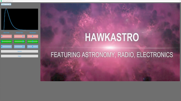
Histogram Matching Application

PLEASE NOTE: the above application is just for experimental purposes and is not suitable for other use. Do not ask for a copy - unless you like being offended by a non-response :-)

The application allowed the generation of a target histogram with various rise-times and delays in terms of their shapes. Two examples are given below...

Using Cumulative Distribution Functions to Match Histograms

The process is as follows...

1. Calculate histogram of original linear image. The data is processed in 16-bit unsigned values - so there are 65536 values in the histogram.
2. Calculate CDF of the linear histogram - also with 65536 values.
3. Calculate CDF of the generated target histogram (as displayed as examples above).
4. Create a re-mapping table by stepping through the linear image CDF values (for levels 0 - 65535) and reading out the CDF value. Then scan through the CDF of the generated target and find the nearest value to the linear CDF value. The index (0 - 65535) becomes the remapped value.
5. For every pixel in the linear image data, look up the entry in the re-mapping table which corresponds to its value and place in a matched image data set.
6. Display the matched image data.

No optimisation of speed nor determination of the most appropriate generated target histogram has been done. Just 'in principle' experiments.

The result of matching the original linear image data (M42: 2.5 minutes integration Seestar S50) histogram to left-most example given above is shown below.

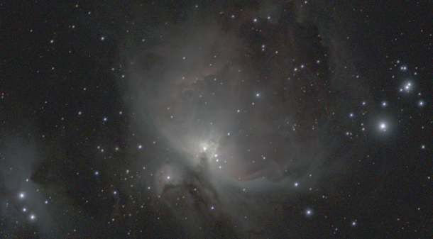
Result of Histogram Matching Using CDF of Generated Target Histogram

Comparing the generated target histogram against the histogram matched linear image shows a close match.

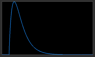
Target Histogram

Linear Data Histogram After Matching

Of note in the 'histogram matched' image is that the low-level nebulosity is visible at the same time as the high level detail (around the Trapezium) is preserved. This is a surprisingly good result. On the downside is the washed-out look in terms of colour. Just why is unknown at the time of writing.

Certainly this is a vast improvement over the previous first attempts at re-mapping using the CDF directly.

Some manipulation in GIMP results in the following image...

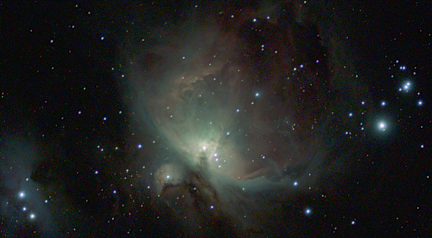
Result of Histogram Matched Image Processed by GIMP

I am pretty pleased with this result.

It may be possible to avoid trying to find the best generated target histogram by analysing good example images of targets and calculating the target histogram directly from those good example images. Perhaps a library of target histograms could be built making post-processing a simple exercise of auto stretching via CDFs with final tweaks in external programs such as GIMP as in the above example.

Interesting...

Histogram Matching...

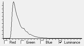
As part of my experiments in astrophotography post-processing I noticed that - after applying a suitable non-linear stretch to the linear image data - the histograms of the stretched image had very similar shapes. As an example the histograms for an image of M42 are shown below.

M42 : Processed (Stretched) Image

The histograms for the luminance and the red, green and blue channels have been separately normalised to better show the similarity in shape. The relative amplitudes of the red, green and blue channels is shown below in the composite histogram plot.

Luminance	Red Channel
Green Channel	Blue Channel
Red, Green and Blue Channels Composite Plot

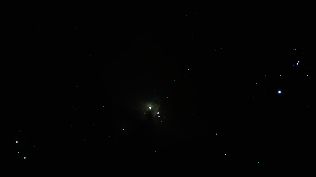
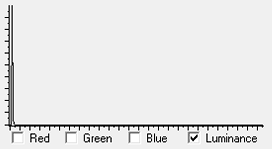
The original linear image as shown below where the pixel values are cramped down at the bottom end as shown in its luminance histogram.

M42: Original Unprocessed Linear Image

Original Linear Image Luminance Histogram

Implementing some way of modifying the data in the original linear image such that its histogram matches the shape and position of a stretched image histogram would be interesting. One way to do that is via "Histogram Matching" - the implementation of which will be described in the next post.

T Coronae Borealis - Recurrent Nova...

Took the opportunity of a clear sky to get a reference image of T Coronae Borealis using the Seestar S50 smart telescope. This is a recurrent nova with a burst period of about 80 years. There was a pre-cursor dimming last year leading to predictions it will go nova sometime this year (2024). Based on past observations it should brighten by a factor of about 1000.

If/when it goes bang I hope to get a comparison image.

Note (added 21 June 2024): I have noticed that in the above image there are 'phantom' stars at the 7 O'clock position next to the bright stars. This is - presumably - due to one or more misaligned sub-frames being added to the stacked image. At a later date a manual stacking process will be used to try and identify the misaligned sub-frames and remove them from the stack.

One-Shot-Colour (OSC) and Debayering...

The sensor in the Seestar S50 is a 'one-shot-colour' (OSC) sensor. Unlike a monochrome sensor - where each pixel in the sensor is a light bucket over a wide range of colours in the spectrum - the OSC sensor has colour filters (red, green and blue) placed over a group of 4 pixels in a 2x2 Bayer matrix. The pattern of filters can vary from sensor to sensor - but in the Seestar S50 the order is GRBG starting from the top-left pixel and moving right - then the second row left-most moving right.

Seestar S50 Bayer Matrix

Note that there are two green pixels in the group of four, with the remaining two red and blue. A number of characteristics arise from this.

• In an image of dimensions W x H, there are (W x H)/2 'green' pixels and (W x H)/4 'red' and 'blue' real physical pixels.
• With three colours in RGB colour space, this number needs to be 'rounded' up to 4 in order to form a symmetrical repeating pattern.
• Green is 'doubled-up' because of the history of OSC sensors is in normal photography and the eye is most sensitive to green.
• In order to provide a value of all three colours for every pixel, a de-bayering (de-mosaicing) algorithm is used. This is a process of generating values from adjacent pixels. There are different de-bayering algorithms and different Bayer matrix ordering. Therefore - when exporting non-debayered image data the Bayer matrix pattern must accompany the data.

In summary - for every 'real' red or 'blue' pixel there are two 'green' pixels. That is, the 'real' resolution for green is twice that of red or blue. This can be seen in the image data.

To illustrate that I've taken a small tile of an image (outlined in red) from the Seestar S50 and examined it in detail. The data is from an image which has been 'stretched' using a CDF (cumulative density function) as described here.

The tile shown below is 25 x 25 pixels and is taken from an area of noisy data. The image data is displayed starting with the RGB composite, then the red, green and blue component magnitudes in row/column order.

What is immediately obvious is that the spatial resolution is much better in the Green channel. The Red and Blue channels are more 'blobby'. In other words - there is more high frequency data (detail) in the Green channel versus the Red and Blue channels.

It can be seen that there are areas in the red and blue data where the level is 'black'. In the corresponding areas in the green data there is fine features. When combined into the RGB composite this is the source of the 'green noise'.

It is interesting to see the effects of 'modulating' the red and blue data with the higher resolution green data. The results are shown below.

Here more detail has been added to the red and blue channels by multiplying their original values by the green channel data. The effect on the original image is shown below.

There is significantly more 'sharpness' in the detail - albeit with corruption of the colour balance. Nonetheless I find this an intriguing result.